Home |
Publications |
Blog
← Back to Blog
Notes
To better understand how modern language models work I figured I would start with the exercise of building a transformer from scratch.
For this exercise I was only allowed to consult the original paper, forums for pytorch / coding related questions and any blog posts on the topic.
I tried to spend as much time building the model from the paper without looking anything up, particularly the tensor math in the attention blocks.
I will be building a 3-layer multi-head attention transformer with an encoder-decoder structure directly from the
Vaswani et al., 2017 paper. I will be using the Opus books english-spanish translation dataset.
Here are some useful resources I found helpful for this process:
I am also including some of the annotated notes I took while reading and trying to visualize the attention heads.
Building a Transformer from Scratch with PyTorch
The code and illustrator files used in this post can be found here: [Illustrator files] and [Transformer Code].
Key Contribution
Before Transformers, Recurrent Neural Networks (RNNs), Long Short-Term Memory (LSTMs), and sometimes Convolutional Neural Networks (CNNs) were used
for sequence modelling and transduction tasks. These models tend to factor computation along the symbol positions of input and output sequences [1].
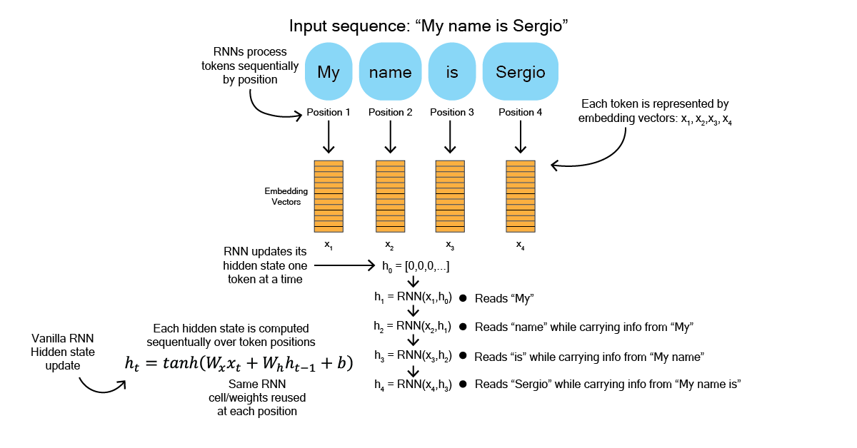
This means that recurrent models break the work of processing a sequence into steps over token positions. A model like an RNN organizes its computation
as a chain across sequence positions, where each token's computations a function of the previous token's hidden state [Figure 1]. Take this example here:
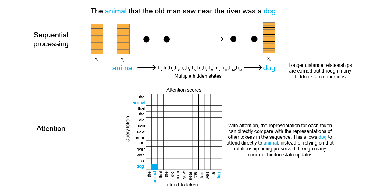
In the above example you can imagine how the amount of processing time would grow in proportion to the numnber of tokens in a sequence. This might not be the most efficient way to process text. This is where attention can be helpful. Attention enables modelling of dependencies without regard to their distances in the input or output sequences [1]. This means that attention enables a model to connect any two tokens in a sequence, even if they are far apart. Take the sentence in [Figure 2] for example.
In summary, attention allows models flexilby focus on relevant tokens anywhere in the input or output sequence, rather than relying on nearby tokens or step-by-step recurrence. Attention therefore facilitates more parallelization and much faster computation. In 2017, Transformers were the only models to rely entirely on self-attention. Before moving onto to the model architecture I found it a useful exercise to unpack how attention is computed, given how important it is here.
Attention
The original transformer is made up of multiple repeating encoder and decoder blocks. Encoder blocks contain a multi-head attention sub-layer and a fully connected feedforward sublayer as well as residual connections and layer norm. Decoder blocks contain the same sublayers but its self-attention uses a causal mask, which prevents each token from attending to future tokens in the decoder input sequence. The decoder also has a third sublayer,a cross-attention block that uses the encoder's output as its source of keys and values. What is a multi-head attention block? In the paper authors state that one of the benefits to the transformer is a reduction in the number of sequential operations required to connect information across positions. However, a single attention head combines information from different token positions into one weighted average. Multi-head attention helps counteract this by allowing the model to attend to different relationships, positions, and representational subspaces in parallel. Let's start by looking at a single attention head and then expanding to include multiple heads.
In the paper, attention is given by:
$ \mathrm{Attention}(Q, K, V) = \mathrm{softmax}\left( \frac{QK^{\top}}{\sqrt{d_k}} \right)V $
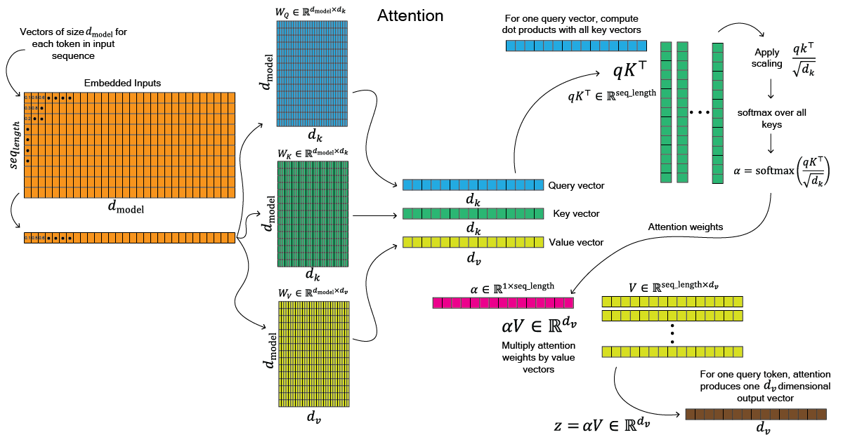
where $Q$, $K$, and $V$ are the query key and value matrices respectively. Before unpacking the matrix multiplication, we can unpack how attention is computed for a single token to all other tokens. After embedding a sequence of tokens, our inputs to the model (the orange matrix in [Figure 3]) are size $seq_{length}$ x $d_{model}$. Attention is computed in parallel for all tokens in the sequence to every other token in the sequence. If we take a single token's input vector the first step is to multiply this input vector by three weight matrices, one for queries ($W_Q$ - blue matrix), one for keys ($W_K$ - green matrix), and one for values ($W_V$ - yello matrix). The query and key weights are size $d_{model}$ x $d_k$, and the value weights are $d_{model}$ x $d_v$. Output of this gives us our $Q$, $K$, and $V$ vectors. To get our attention scores we need to take the dot product of the query and key vectors ($QK^{\top}$, in the attention equation). For a single query token, this is $qK^{\top}$ which gives us a vector that is $\in \mathbb{R}^{{seq_{length}}}$ which we then scale by $\sqrt{d_k}$. We then compute the softmax over all keys which guves us our attention weights for a single query vector (pink vector, $\alpha$). Finally we multiple these attention weights by our Value vectors to get, $\alpha V \in \mathbb{R}^{d_v}$. This output vector is size $d_v$.
Another way to view this is our current token carries a query, like a question it wants answered. Every token in the sequence carries a key, like a name tag describing what kind of information it has. Each token also has a value, which is the actual information it can contribute. The query is compared (dot product) with each key to produce a relevance score. After scaling and softmax, these scores become attention weights: how much the token should “listen” to each other token. Finally, the token forms its new representation by taking a weighted mixture of the value vectors. So for for this query token's we have generated a sort of context-aware representation.
Tensor Math
In practice, these functions are implemented with tensors using:
$ \mathrm{MultiHead}(Q, K, V) = \mathrm{Concat}(\mathrm{head}_1, \ldots, \mathrm{head}_h) W^O \\ \text{where }
\mathrm{head}_i = \mathrm{Attention}\left(QW_i^Q,\,KW_i^K,\,VW_i^V\right)$
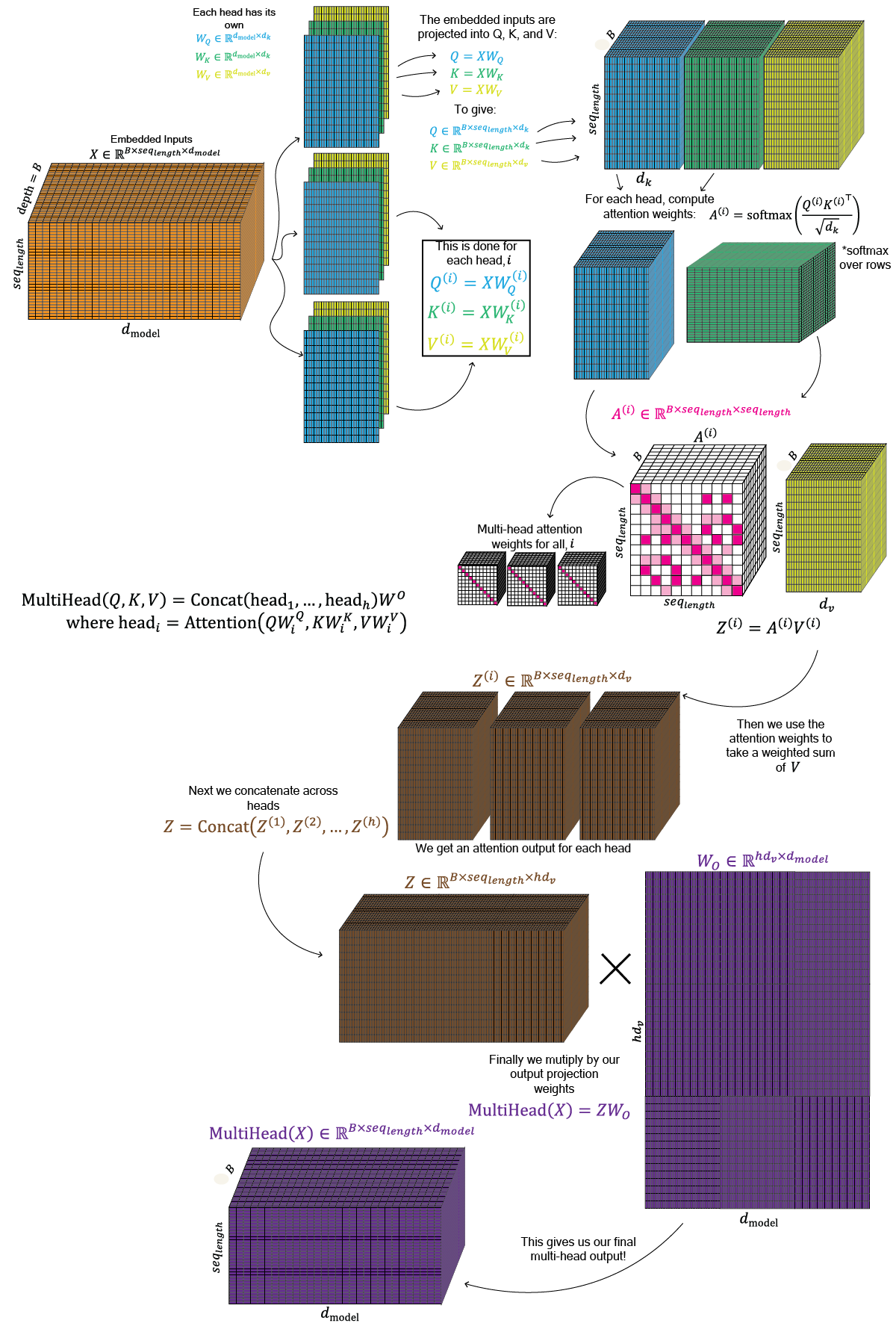
Our actual inputs to the model look something like the input tensor in [Figure 4], and are size $batch_{size}$ x $seq_{length}$ x $d_{model}$ , where $B$ is the batch size. In multi-head attention, each head has its own projection matrices $W_Q^{(i)}$, $W_K^{(i)}$, and $W_V^{(i)}$, which project the input embeddings into query, key, and value tensors. For a single head, $Q^{(i)}$, $K^{(i)}$, and $V^{(i)}$ and have shape $B$ x $seq_{length}$ x $d_k$ (& $d_v$). These are usually represented as $B$ x $n_{heads}$ x $seq_{length}$ x $d_k$ (& $d_v$)
For each head, we compute the attention weights: $A^{(i)} = \mathrm{softmax}\left(\frac{Q^{(i)}K^{(i)\top}}{\sqrt{d_k}}\right)$. This gives us $A$, which across all heads,has shape $B$ x $n_{heads}$ x $seq_{length}$ x $seq_{length}$. We then use these attention weights to take a weighted sum of the value vectors, giving the head outputs $V$. $Z = AV$, which have shape $B$ x $n_{heads}$ x $seq_{length}$ x $d_v$. Finally, we concatenate the head outputs along the feature dimension, producing a tensor of shape, $B$ x $seq_{length}$ x $n_{heads}*d_v$ and multiply by the output projection matrix $W_O$ so that the final output returns to shape $batch_{size}$ x $seq_{length}$ x $d_{model}$.
Multi-head attention lets the model compare every token to every other token in several different ways at once. Each head computes its own attention pattern, uses it to mix information across tokens, and then all head outputs are combined back into one representation.
Now that I have reviewed attention, I think it is safe to move on to building our transformer step by step. I am going to go out of order from the paper and in the order of sublayers in the model. We will start with the embeddings.
Embeddings
The embedding layer in a transformer at a high level, takes tokens as inputs and converts them to dense vector-based representations. In practice the input tokens may be $batch_{size}$ x $seq_{length}$. The embedding weights are $Vocab Size$ x $d_{model}$. We can use our tokens to index the embedding weights giving us a tensor with shape $batch_{size}$ x $seq_{length}$ x $d_{model}$. These representations are useful because they capture the statistical relationships between tokens being embedded. They are able to do this because these vectors are learned during training. I.e., At the start of training, an embedding vector is basically random. The model does not know that "cat" and "dog" are related. But during training, the model repeatedly sees tokens in contexts and updates the embedding vectors to make better predictions. "The cat ate food" and "The dog ate food", have "cat" and "dog" appear similar contexts, so the model may learn to give them somewhat similar vector representations.
I used cosine similarity to compare vectors after training my smaller model and you can see some simple relationships.
Terminal Output:

Pair: a, an | Counts: 2373 , 366 | Cosine Similarity: 0.6951920986175537
Pair: not, t | Counts: 1043 , 309 | Cosine Similarity: 0.626957356929779
Pair: from, of | Counts: 413 , 2590 | Cosine Similarity: 0.5721158981323242
Pair: ;, , | Counts: 665 , 9004 | Cosine Similarity: 0.5594618916511536
Pair: exclaimed, cried | Counts: 53 , 145 | Cosine Similarity: 0.5560516119003296
Pair: not, nothing | Counts: 1043 , 177 | Cosine Similarity: 0.5434814095497131
Pair: i, me | Counts: 2732 , 714 | Cosine Similarity: 0.5395011305809021
Pair: un, a | Counts: 52 , 2373 | Cosine Similarity: 0.5394478440284729
Pair: !, ? | Counts: 1429 , 1563 | Cosine Similarity: 0.5386260747909546
Pair: de, of | Counts: 134 , 2590 | Cosine Similarity: 0.5383878350257874
Pair: t, no | Counts: 309 , 579 | Cosine Similarity: 0.5358028411865234
Pair: s, of | Counts: 627 , 2590 | Cosine Similarity: 0.5356942415237427
Pair: she, he | Counts: 685 , 1637 | Cosine Similarity: 0.5340654253959656
Pair: not, no | Counts: 1043 , 579 | Cosine Similarity: 0.5280725359916687
Pair: !, ; | Counts: 1429 , 665 | Cosine Similarity: 0.5189635753631592
Pair: the, un | Counts: 6218 , 52 | Cosine Similarity: 0.5146258473396301
Pair: answered, replied | Counts: 78 , 221 | Cosine Similarity: 0.5123234987258911
Pair: said, exclaimed | Counts: 904 , 53 | Cosine Similarity: 0.5095114707946777
Pair: which, that | Counts: 475 , 1501 | Cosine Similarity: 0.5090993642807007
Pair: his, her | Counts: 1088 , 678 | Cosine Similarity: 0.5075424313545227
Pair: -, : | Counts: 1191 , 310 | Cosine Similarity: 0.5046187043190002
Pair: replied, said | Counts: 221 , 904 | Cosine Similarity: 0.5028983950614929
Pair: are, thou | Counts: 434 , 47 | Cosine Similarity: 0.4969075918197632
Pair: said, answered | Counts: 904 , 78 | Cosine Similarity: 0.4963621497154236
Pair: myself, me | Counts: 82 , 714 | Cosine Similarity: 0.49230483174324036
Pair: i, myself | Counts: 2732 , 82 | Cosine Similarity: 0.4877903461456299
Pair: -, ; | Counts: 1191 , 665 | Cosine Similarity: 0.48768070340156555
Pair: no, nothing | Counts: 579 , 177 | Cosine Similarity: 0.48696935176849365
Pair: his, the | Counts: 1088 , 6218 | Cosine Similarity: 0.48408859968185425
Pair: ", — | Counts: 6788 , 72 | Cosine Similarity: 0.4839264750480652
Pair: this, a | Counts: 724 , 2373 | Cosine Similarity: 0.4830649197101593
Pair: his, your | Counts: 1088 , 370 | Cosine Similarity: 0.4816626012325287
Pair: his, their | Counts: 1088 , 228 | Cosine Similarity: 0.47955596446990967
Pair: fear, qu | Counts: 37 , 37 | Cosine Similarity: 0.4762763977050781
Pair: is, are | Counts: 1144 , 434 | Cosine Similarity: 0.4740842282772064
Pair: et, , | Counts: 68 , 9004 | Cosine Similarity: 0.4727495014667511
This is a smaller model so these examples might not be super semantically rich, despite this you do see some things like function-word pairs (i.e., "a" and "an", "is" and "are", "from" and "of"), pronoun clusters (i.e., "he", and "she", "his" and "her"), and some words that seem to be related to dialogue (i.e., "said", "exclaimed", "answered", "replied"). This suggests that even in a smaller model the embeddings are capturing some of the statistical relationships between tokens.
Embedding Code
Here is the code [GitHub - Embedding.py] to build the embedding layer. We initialize the embedding weights with size $Vocab_{size}$ x $d_{model}$ and subsequently pass tokens as indices to the embedding matrix.
The paper also multiplies the embeddings by $\sqrt{d_{model}}$ to scale them.
class Param:
    vocab_size: int = 1000
    d_model: int = 128
    batch_size: int  = 16
    seq_len: int = 32

param = Param() # Initialize some parameters

class Embedding(nn.Module):
    def __init__(self, param):
        super().__init__()
        self.param = param
        self.WE = nn.Parameter(torch.randn(self.param.vocab_size, self.param.d_model)) # Initialize embedding weights

    def forward(self, tokens):
        # Index embedding weights with input tokens and scale by sqrt(d_model)
        return self.WE[tokens] * math.sqrt(self.param.d_model)

tokens = torch.randint(0, param.vocab_size, (param.batch_size, param.seq_len)) # Initialize random tokens
emb = Embedding(param) # Initialize the embedding layer
embeddings = emb(tokens) # Pass the tokens through the embedding layer

print(f'Input Tokens with shape: {tokens.shape}') # (Batch Size, Sequence Length)
print(f'Embeddings with shape: {embeddings.shape}') # (Batch Size, Sequence Length, D_Model)
Terminal Output:

Input Tokens with shape: torch.Size([16, 1000])
Embeddings with shape: torch.Size([16, 1000, 512])
Positional Encoding
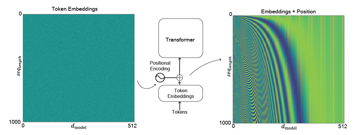
There is another step to the embedding process prior to feeding the input into the transformer layers. Because there is no recurrent in order for the model to know the order of tokens there has to be some information bout where token is in a sequence (it's positional encoding). Therefore they positional encoding which is the same size as the embeddings, $seq_{length}$ x $d_{model}$. Positional encodings can be given in many ways, but in the paper they use:
$PE_{(pos, 2i)} = \sin\left(\frac{pos}{10000^{2i/d_{\text{model}}}}\right) \\ PE_{(pos, 2i+1)} = \cos\left(\frac{pos}{10000^{2i/d_{\text{model}}}}\right)$
Where $pos$ is the position of the token in the sequence and $i$ is the index of the dimension in the embedding. This works because each position gets a mixture of sine and cosine waves at slightly different frequencies. Importantly models can distinguish between different positions while keep information about distances.
Positional Encoding Code
Here is the code [GitHub - PositionalEncoding.py] to implement positional encoding:
        class Param:
    vocab_size: int = 1000
    d_model: int = 512
    batch_size: int  = 16
    seq_len: int = 1000
    init_scale: float = 0.02

param = Param() # Initialize some parameters

class PositionEmbed(nn.Module):
    def __init__(self,param):
        super().__init__()
        self.param = param
        PE = torch.empty(self.param.seq_len,self.param.d_model) # Create an empty tensor for positional encodings
        pos = torch.arange(0,self.param.seq_len)[:,None] # Create a tensor of shape (seq_len, 1) with position indices
        dim = torch.arange(0,self.param.d_model,2) # Create a tensor of shape (d_model/2,) with even dimension indices
        denom = torch.exp(dim * (-math.log(10000) / self.param.d_model)) # Calculate the denominator for the sine and cosine functions
        PE[:,0::2] = torch.sin(denom * pos) # Apply sine to even dimensions
        PE[:,1::2] = torch.cos(denom * pos) # Apply cosine to odd dimensions
        self.register_buffer("PE", PE) # Register PE as a buffer so it is not updated during training but is saved with the model

    def forward(self,embedded):
        return embedded + self.PE # Simply add the positional encoding to the input embeddings.

embeddings = torch.randn(param.batch_size, param.seq_len, param.d_model)*param.init_scale # Init random embeddings
pos = PositionEmbed(param) # Initialize the positional encoding layer
pos_embeddings = pos(embeddings) # Add positional encodings to the embeddings

print(f'Input Embeddings with shape: {embeddings.shape}') # (Batch Size, Sequence Length, D_Model)
print(f'Positional Embeddings with shape: {pos_embeddings.shape}') # (Batch Size, Sequence Length, D_Model)
Terminal Output:

Input Embeddings with shape: torch.Size([16, 1000, 512])
Positional Embeddings with shape: torch.Size([16, 1000, 512])
Now we have our inputs to the transformer, the next step is to implement the attention blocks.
Attention Blocks
As mentioned before, both the encoder and decoder blocks contain multi-head attention sublayers.
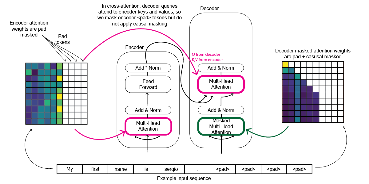
The difference between the encoder and decoder attention is that the decoder uses a causal mask to prevent tokens from attending to future tokens in the decoder input sequence. The decoder also has a third sublayer, a cross-attention block that uses the encoder's output as its source of keys and values. We can write our attention code to handle all three instances of attention in the model. The inputs to our attention multihead attention blocks are the same size as the output of the embedding layer, $batch_{size}$ x $seq_{length}$ x $d_{model}$. The output of the attention blocks is also the same size, so that it can be passed to the next layer. This is also where we get to apply our tensor math from before [Figure 4]. Our attention code will initilize trainable weights for the query, key, and valye projections. These will be size $d_{model}$ x $d_k$ for the query and key projections and $d_{model}$ x $d_v$ for the value projections. We will also initialize an output projection matrix of size $n_{heads}*d_v$ x $d_{model}$. In the forward pass we will compute the attention scores, apply the softmax to get attention weights, and then use these weights to take a weighted sum of the value vectors. Finally we will concatenate the head outputs and pass them through the output projection matrix to get our final output.
Attention Code
Here is the code [GitHub - MultiHeadAttention.py] to implement multi-head attention:
    import torch
import torch.nn as nn
import math
import matplotlib.pyplot as plt
import numpy as np

class Param:
    h: int = 2
    vocab_size: int = 1000
    d_model: int = 512
    batch_size: int  = 16
    seq_len: int = 1000
    d_k: int = 64
    d_v: int = 64
    init_scale: float = 0.02

param = Param() # Initialize some parameters

class MultiHeadAttention(nn.Module):
    def __init__(self,param):
        super().__init__()
        self.param = param
        # initialize the weight and bias parameters for the query, key, value, and output projections
        # WQ & WK Shape: # shape (h, d_model, d_k)
        self.WQ = nn.Parameter(torch.randn(self.param.h,self.param.d_model,self.param.d_k)*self.param.init_scale)
        self.bQ = nn.Parameter(torch.ones(self.param.h,self.param.d_k)) # shape (h, d_k)
        self.WK = nn.Parameter(torch.randn(self.param.h,self.param.d_model,self.param.d_k)*self.param.init_scale)
        self.bK = nn.Parameter(torch.ones(self.param.h,self.param.d_k)) # shape (h, d_k)
        # WV Shape: # shape (h, d_model, d_v)
        self.WV = nn.Parameter(torch.randn(self.param.h,self.param.d_model,self.param.d_v)*self.param.init_scale)
        self.bV = nn.Parameter(torch.ones(self.param.h,self.param.d_v)) # shape (h, d_v)
        # WO Shape: # shape (h * d_v, d_model)
        self.WO = nn.Parameter(torch.randn(self.param.h * self.param.d_v,self.param.d_model)*self.param.init_scale)
        self.bO = nn.Parameter(torch.ones(self.param.d_model)) # output projection bias # shape (h, d_model)

    def forward(self,resid,padding_mask=None,causal_mask = False,crs_input=None):
        # Q, K, V projections for all heads in parallel
        # shapes: Q: (batch_size, h, seq_len, d_k) & (batch_size, h, seq_len, d_v)
        Q = resid[:,None,:,:] @ self.WQ[None,:,:,:] + self.bQ[None,:,None,:]
        if crs_input is not None:
            K = crs_input[:,None,:,:] @ self.WK[None,:,:,:] + self.bK[None,:,None,:]
            V = crs_input[:,None,:,:] @ self.WV[None,:,:,:] + self.bV[None,:,None,:]
        else:
            K = resid[:,None,:,:] @ self.WK[None,:,:,:] + self.bK[None,:,None,:]
            V = resid[:,None,:,:] @ self.WV[None,:,:,:] + self.bV[None,:,None,:]
        attn = Q @ K.transpose(-2,-1) / math.sqrt(self.param.d_k) # shape (batch_size, h, seq_len, seq_len)
        if padding_mask is not None:
            attn = torch.masked_fill(attn, padding_mask, -torch.inf)
        if causal_mask: # apply causal mask to attention scores
            mask = MultiHeadAttention.causal_mask(self) # shape (1, 1, seq_len, seq_len)
            attn = torch.masked_fill(attn,mask,-torch.inf)
        attn = attn.softmax(dim=-1) # softmax **After applying masks
        out = attn @ V # shape (batch_size, h, seq_len, d_v)
        # concatenate the outputs of the attention heads and apply the output projection
        concatenated = out.transpose(1,2).reshape(resid.shape[0], resid.shape[1], self.param.h * self.param.d_v)
        out = concatenated @ self.WO + self.bO[None,None,:]
        return out, attn # return attn head outputs

    @staticmethod
    def padding_mask(tokens,pad_id):
        mask = (tokens==pad_id)[:,None,None,:] # broadcast across each column in each head
        return mask

    def causal_mask(self):
        mask = ~torch.tril(torch.ones((self.param.seq_len,self.param.seq_len))).bool() # shape (seq_len, seq_len)
        return mask

embeddings = torch.randn(param.batch_size, param.seq_len, param.d_model)
# pretend last 6 tokens in first sequence are padding
tokens = torch.ones(param.batch_size, param.seq_len).long()
tokens[0, -6:] = 0
mha = MultiHeadAttention(param) # initilize multi-head attention
padding_mask = MultiHeadAttention.padding_mask(tokens, pad_id=0) # padding mask

out, attn = mha(embeddings,padding_mask=padding_mask,causal_mask=False)

print(f'Input shape: {embeddings.shape}') # should be (batch_size, seq_len, d_model)
print(f'Attention output shape: {out.shape}') # should be (batch_size, seq_len, d_model)
    Terminal Output:

Input shape: torch.Size([16, 1000, 512])
Attention output shape: torch.Size([16, 1000, 512])
One final note about masking, at a very high level the encoder uses pad masking to ignore padded tokens in the input sequence. The decoder uses both pad masking and causal masking [figure 6]. This is because in the paper they state: In "encoder-decoder attention" layers, the queries come from the previous decoder layer, and the memory keys and values come from the output of the encoder. As well as: Similarly, self-attention layers in the decoder allow each position in the decoder to attend to all positions in the decoder up to and including that position. We need to prevent leftward information flow in the decoder to preserve the auto-regressive property. [1 - Section 3.2.3]
The next sublayer that the encoding blocks have is the feed-forward sublayer.
Feed-Forward Sublayer
The feed forwad layer is given by:
$FFN(x) = \max(0, xW_1 + b_1)W_2 + b_2$
Both the encoder and decoder blocks contain a position-wise feedforward network. The layer is made up of two linear transformations with a ReLU activation in between. The first linear transformation takes the output of the attention sublayer (after residual connection and layer norm) which are size $batch_{size}$ x $seq_{length}$ x $d_{model}$ and projects them up to a higher dimensional space, $batch_{size}$ x $seq_{length}$ x $d_{ff}$. The second linear transformation projects this back down to the original dimension, $batch_{size}$ x $seq_{length}$ x $d_{model}$. This feedforward network is applied independently to each position in the sequence. The purpose of this sublayer is to introduce non-linearity and allow the model to learn more complex transformations of the data after the attention sublayer has mixed information across tokens.
Small note on ReLU
In the original paper they use a ReLU to introduce non-linearity. Nowadays, other activation functions like GELUs [2] are also commonly used. I think in general the important part of this is that it let's the model be slightly more expressive than a linear transformation.
Feed-Forward Code
Here is the code [GitHub - FeedForward.py] to implement the feed-forward sublayer:
    import torch
import torch.nn as nn
import math

class Param:
    h: int = 2
    vocab_size: int = 1000
    d_model: int = 512
    batch_size: int  = 16
    seq_len: int = 1000
    d_k: int = 64
    d_v: int = 64
    d_ff: int = 2048 # feedforward hidden dimension
    init_scale: float = 0.02

param = Param() # initialize some params

class FeedForward(nn.Module):
    def __init__(self,param):
        super().__init__()
        self.param = param
        # Initialize hidden layers weights and biases for the feedforward network
        # WH shape (d_model, d_ff)
        self.WH = nn.Parameter(torch.randn(self.param.d_model,self.param.d_ff)*self.param.init_scale)
        self.bH = nn.Parameter(torch.ones(self.param.d_ff)) # shape (d_ff,)
        # initialize output projection weights and biases for the feedforward network
        # WO shape (d_ff, d_model)
        self.WO = nn.Parameter(torch.randn(self.param.d_ff,self.param.d_model)*self.param.init_scale)
        self.bO = nn.Parameter(torch.ones(self.param.d_model)) # shape (d_model,)

    def forward(self,resid):
        return torch.relu(resid @ self.WH + self.bH) @ self.WO + self.bO

residual = torch.randn(param.batch_size, param.seq_len, param.d_model)
ff = FeedForward(param)
ff_out = ff(residual)

print(f'Input shape: {residual.shape}') # should be (batch_size, seq_len, d_model)
print(f'Feedforward output shape: {ff_out.shape}') # should be (batch_size, seq_len, d_model)
    Terminal Output:
Input shape: torch.Size([16, 1000, 512])
Feedforward output shape: torch.Size([16, 1000, 512])
We have built much of what we need for both the encoder and decoder. There is one repeating component that we will implement next. These are the add + norm layers in the model.
Residual Connections and Layer Normalization
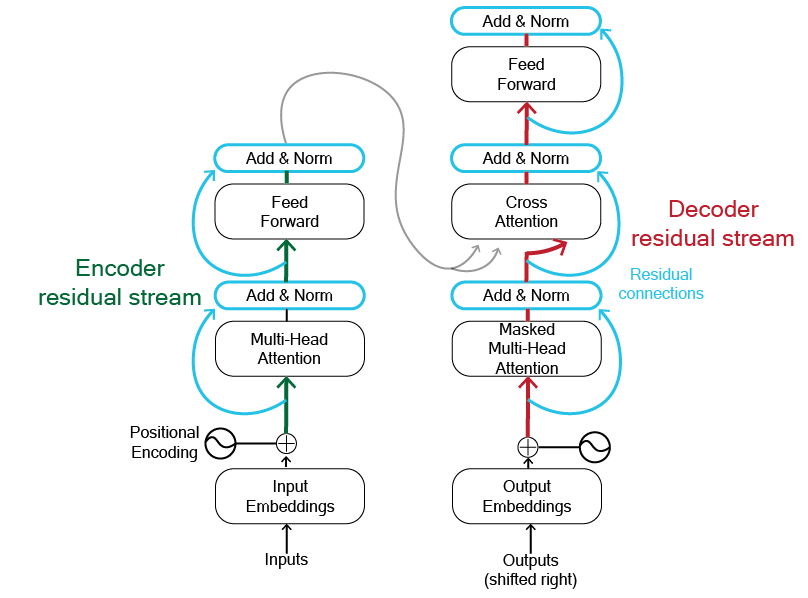
One of the main components of the transformer architecture is the use of residual connections each layer has. These connections [Figure 7] take the input to a layer and add it to the output of the same layer before normalization. Another way to understand this is as "read" and "write" operations where the input is read and written (added) to the output again [3].
Layer normalization is implemented as in [4]. Layer norm get's applied after each sublayer such that, $LayerNorm(x + sublayer(x))$. We will build the residual stream connections into the encoder and decoder blocks.
Layer Normalization Code
Here is the code [GitHub - LayerNorm.py] to implement layer normalization:
    import torch
import torch.nn as nn

print('\n'*2)
class Param:
    vocab_size: int = 1000
    d_model: int = 512
    batch_size: int  = 16
    seq_len: int = 1000
param = Param() # initialize some params

class LayerNorm(nn.Module):
    def __init__(self,param):
        super().__init__()
        self.param = param
        # scale parameter for layer normalization
        self.gamma = nn.Parameter(torch.ones(param.d_model)) # (d_model,)
        # shift parameter for layer normalization
        self.beta = nn.Parameter(torch.zeros(param.d_model)) # (d_model,)

    def forward(self,x):
        # compute mean across the d_model for each position in the sequence
        mean = x.mean(-1, keepdim=True) # shape (batch_size, seq_len, 1)
        # compute standard deviation across the d_model for each position in the sequence
        std = x.std(-1, keepdim=True) # shape (batch_size, seq_len, 1)
        # normalize (with a small epsilon for numerical stability)
        normalized_x = (x - mean) / (std + 1e-5) # shape (batch_size, seq_len, 1)
        # scale and shift the normalized input using the learnable parameters gamma and beta
        return self.gamma * normalized_x + self.beta

residual = torch.randn(param.batch_size, param.seq_len, param.d_model) # random tensor
ln = LayerNorm(param) # initialize the layer normalization layer
ln_out = ln(residual) # apply layer normalization to the residual input

print(f'Residual input shape: {residual.shape}') # should be (batch_size, seq_len, d_model)
print(f'LayerNorm output shape: {ln_out.shape}') # should be (batch_size, seq_len, d_model)
    Terminal Output:

Residual input shape: torch.Size([16, 1000, 512])
LayerNorm output shape: torch.Size([16, 1000, 512])
Now that we have built everthing we need for the encoder and decoder blocks we can build each of them. We will start with the encoder blocks.
Encoder Blocks
The encoder blocks are made up of two sublayers, a multi-head self-attention layer and a feed-forward layer. They take the source tokens as inputs (which are differnet than the target tokens that the decoder takes as inputs). The input embeddings are size $batch_{size}$ x $seq_{length}$ x $d_{model}$ and the output of each sublayer is also size $batch_{size}$ x $seq_{length}$ x $d_{model}$. For the encoder we need to give the source inputs and source padding mask. We will build an encoder module as well as the encoder blocks, which are just stacked encoders. The output from the previous encoder block becomes the input to the next encoder block.
Encoder Block Code
Here is the code [GitHub - Encoder.py] to implement the encoder blocks:
    from MultiHeadAttention import MultiHeadAttention
from FeedForward import FeedForward
from LayerNorm import LayerNorm
import torch
import torch.nn as nn

class Param:
    N: int = 2 # number of encoder and decoder blocks
    h: int = 2
    vocab_size: int = 1000
    d_model: int = 512
    batch_size: int  = 16
    seq_len: int = 1000
    d_k: int = 64
    d_v: int = 64
    d_ff: int = 2048 # feedforward hidden dimension
    init_scale: float = 0.02
param = Param()

class Encoder(nn.Module):
    def __init__(self,param):
        super().__init__()
        self.param = param
        self.attn = MultiHeadAttention(param) # multi-head self attention layer
        self.ff = FeedForward(param) # feedforward layer
        self.ln1 = LayerNorm(param) # layer normalization after attention
        self.ln2 = LayerNorm(param) # layer normalization after feedforward

    def forward(self,resid,src_padding_mask):
        x, attn = self.attn(resid,padding_mask=src_padding_mask,causal_mask=False)
        resid = self.ln1(resid + x) # LayerNorm1(add residual)
        x = self.ff(resid) # feed forward layer
        return self.ln2(resid + x) # LayerNorm2(add residual)

class EncoderStack(nn.Module):
    def __init__(self,param):
        super().__init__()
        self.param = param
        # Create a stack of N encoder blocks using nn.ModuleList to hold the encoder layers.
        # Each encoder is initialize with the same parameters
        self.encoders = nn.ModuleList([Encoder(self.param) for _ in range(self.param.N)])

    def forward(self,resid,src_padding_mask):
        # The output of one encoder block becomes the input to the next encoder block.
        for enc in self.encoders:
                resid = enc(resid,src_padding_mask=src_padding_mask)
        return resid

resid = torch.randn(param.batch_size, param.seq_len, param.d_model) # random tensor input to encoder stack
# no padding mask for this test
encoder_stack = EncoderStack(param) # initialize encoder stack
encoder_out = encoder_stack(resid, src_padding_mask=None) # forward pass through encoder stack

print(f'Encoder input shape: {resid.shape}') # should be (batch_size, seq_len, d_model)
print(f'Encoder stack output shape: {encoder_out.shape}') # should be (batch_size, seq_len, d_model)
    Terminal Output:

Encoder input shape: torch.Size([16, 1000, 512])
Encoder stack output shape: torch.Size([16, 1000, 512])
Next we can implement the decoder.
Decoder Blocks
The decoder blocks are made up of three sublayers, a multi-head self-attention layer, a multi-head cross-attention layer, and a feed-forward layer. The inputs and outputs to each sublayer are $batch_{size}$ x $seq_{length}$ x $d_{model}$. We also have to take the outputs from the encoder stack as inputs to the cross-attention layer in each decoder. The input embeddings are the different from the source embeddings, they are the target embeddings. We also ensure for the masked multi-head attention we set causal mask to true.
Decoder Blocks Code
Here is the code [GitHub - Decoder.py] to implement the decoder blocks:
    from MultiHeadAttention import MultiHeadAttention
from FeedForward import FeedForward
from LayerNorm import LayerNorm
from Encoder import EncoderStack
import torch
import torch.nn as nn

class Param:
    N: int = 2 # number of encoder and decoder blocks
    h: int = 2
    vocab_size: int = 1000
    d_model: int = 512
    batch_size: int  = 16
    seq_len: int = 1000
    d_k: int = 64
    d_v: int = 64
    d_ff: int = 2048 # feedforward hidden dimension
    init_scale: float = 0.02
param = Param()

class Decoder(nn.Module):
    def __init__(self,param,):
        super().__init__()
        self.param = param
        self.attn = MultiHeadAttention(param) # multi-head self attention layer
        self.crs_attn = MultiHeadAttention(param) # multi-head cross attention layer
        self.ff = FeedForward(param) # feedforward layer
        self.ln1 = LayerNorm(param) # layer normalization after self attention
        self.ln2 = LayerNorm(param) # layer normalization after cross attention
        self.ln3 = LayerNorm(param) # layer normalization after feedforward

    def forward(self,resid,tgt_padding_mask,src_padding_mask,crs_input):
        x, self_attn = self.attn(resid,padding_mask=tgt_padding_mask)
        resid = self.ln1(resid + x)
        x, crs_attn = self.crs_attn(resid,padding_mask=src_padding_mask,causal_mask=False,crs_input=crs_input)
        resid = self.ln2(resid + x)
        x = self.ff(resid)
        return self.ln3(resid + x)

class DecoderStack(nn.Module):
    def __init__(self,param):
        super().__init__()
        self.param = param
        # Create a stack of N decoder blocks using nn.ModuleList to hold the decoder layers
        # Each decoder is initialize with the same parameters
        self.decoders = nn.ModuleList([Decoder(self.param) for _ in range(self.param.N)])

    def forward(self,resid,tgt_padding_mask,src_padding_mask,crs_input):
        for dec in self.decoders:
            # The output of one encoder block becomes the input to the next encoder block.
            resid = dec(resid,tgt_padding_mask=tgt_padding_mask,src_padding_mask=src_padding_mask,crs_input=crs_input)
        return resid

resid = torch.randn(param.batch_size, param.seq_len, param.d_model) # random tensor decoder input
tgt_padding_mask = None # no padding mask for this test
src_padding_mask = None # no padding mask for this test
encoder_stack = EncoderStack(param)
crs_input = encoder_stack(input, src_padding_mask) # output from encoder stack to be used as cross attention input
decoder_stack = DecoderStack(param)
decoder_out = decoder_stack(resid,tgt_padding_mask,src_padding_mask,crs_input) # forward pass through decoder stack

print(f'Decoder Input shape: {resid.shape}') # should be (batch_size, seq_len, d_model)
print(f'Cross attention input shape: {crs_input.shape}') # should be (batch_size, seq_len, d_model)
print(f'Decoder stack output shape: {decoder_out.shape}') # should be (batch_size, seq_len, d_model)
    Terminal Output:

Dcoder input shape: torch.Size([16, 1000, 512])
Cross attention input shape: torch.Size([16, 1000, 512])
Decoder stack output shape: torch.Size([16, 1000, 512])
Lastly we have one more step before we can put all the pieces together in a Transformer class. We need to build the unembedding layer to convert the decoder output into logits for each token in the vocabulary. Because I want to know, what is the next token!
Unembedding Layer
The unembedding layer is a simple linear layer that takes the output of the decoder and projects it the size of the vocabulary. This is done by initializing unembedding weights size $d_{model}$ x $vocab_{size}$. The output of the unembedding layer is size $batch_{size}$ x $seq_{length}$ x $vocab_{size}$. This gives us the logits for each token in the vocab. We can then apply a softmax to these logits to get probabilities for each token.
Unembedding Code
Here is the code [GitHub - Unembed.py] to implement the unembedding layer:
    import torch
import torch.nn as nn

print('\n'*2)
class Param:
    h: int = 2
    vocab_size: int = 1000
    d_model: int = 512
    batch_size: int  = 16
    seq_len: int = 1000
    d_k: int = 64
    d_v: int = 64
    init_scale: float = 0.02
param = Param()

class Unembed(nn.Module):
    def __init__(self,param):
        super().__init__()
        self.param = param
        # initialize unembedding weights and bias
        self.WU = nn.Parameter(torch.randn(self.param.d_model,self.param.vocab_size)*self.param.init_scale) # (d_model, vocab_size)
        self.bU = nn.Parameter(torch.ones(self.param.vocab_size)) # (vocab_size,)

    def forward(self,resid):
        logits = resid @ self.WU[None,:,:] + self.bU # shape (batch_size, seq_len, vocab_size)
        probs = logits.softmax(dim=-1) # shape (batch_size, seq_len, vocab_size)
        return logits, probs

decoder_output = torch.randn(param.batch_size, param.seq_len, param.d_model) # random tensor decoder output
unembed = Unembed(param) # initialize unembedding layer

logits, probs = unembed(decoder_output) # get logits and probabilities for each token
print(f'Unembedding output shape (logits): {logits.shape}') # should be (batch_size, seq_len, vocab_size)
print(f'Unembedding output shape (probs): {probs.shape}') # should be (batch_size, seq_len, vocab_size)
    Terminal Output:

Unembedding input shape (decoder output): torch.Size([16, 1000, 512])
Unembedding output shape (logits): torch.Size([16, 1000, 1000])
We have built all the componenets we need for our transformer model! Now we just need to put all the pieces together in a Transformer class. The TranslationData class is just a helper class to load in the translation data and create the source and target vocabularies. When I run the model for real I will use this to load the hugging face Opus books english-spanish translation dataset. For testing purposes I will just use random tensors as inputs to the model.
The Transformer
Transformer Code
Here is the code [GitHub - Transformer.py] to implement the transformer class:
    from Embedding import Embedding
from PositionalEncoding import PositionEmbed
from MultiHeadAttention import MultiHeadAttention
from FeedForward import FeedForward
from LayerNorm import LayerNorm
from Encoder import EncoderStack
from Decoder import DecoderStack
from Unembed import Unembed
from TranslationData import build_translation_datasets
from torch.utils.data import DataLoader
import torch
import torch.nn as nn

train_dataset, test_dataset = build_translation_datasets(
    dataset_name="opus_books",
    lang_pair="en-es",
    src_lang="en",
    tgt_lang="es",
    max_len=1000,
    max_vocab=10000,
    n_train=10000,
    n_test=1000
)
dataset = train_dataset

class Param:
    N: int = 2 # number of encoder and decoder blocks
    h: int = 2 # number of attention heads
    vocab_size: int = 10000 #same for source and target language for simplicity
    d_model: int = 512 # dimensionality of model (input and output of each sublayer)
    batch_size: int  = 16 # batch size for training
    seq_len: int = 1000 # maximum sequence length (for padding and positional encoding)
    d_k: int = 64 # dimensionality of keys and queries in multi-head attention
    d_v: int = 64 # dimensionality of values in multi-head attention
    d_ff: int = 2048 # feedforward hidden dimension
    lr: float = 1e-4 # learning rate for training
    iters: int = 2000 # number of training iterations
    init_scale: float = 0.02 # scale for initializing weights

param = Param()

class Transformer(nn.Module):
    def __init__(self, param, dataset=None):
        super().__init__()
        self.param = param
        self.dataset = dataset
        self.src_embedding = Embedding(param) # Initiliaze src embedding
        self.tgt_embedding = Embedding(param) # Initialize tgt embedding
        self.pos_embedding = PositionEmbed(param) # Initialize positional embedding
        self.encoder_stack = EncoderStack(param) # Initialize encoder stack (N encoder blocks)
        self.decoder_stack = DecoderStack(param) # Initialize decoder stack (N decoder blocks)
        self.unembed = Unembed(param) # Initialize unembedding layer

    # build the forward pass through the model
    def forward(self,src_tokens,tgt_tokens):
        # create src & tgt padding mask
        src_pad_id = self.dataset.src_stoi[""]
        tgt_pad_id = self.dataset.tgt_stoi[""]
        src_padding_mask = MultiHeadAttention.padding_mask(src_tokens, src_pad_id)
        tgt_padding_mask = MultiHeadAttention.padding_mask(tgt_tokens, tgt_pad_id)
        # embed source tokens and add positional encoding
        src_embedded = self.pos_embedding(self.src_embedding(src_tokens))
        # embed target tokens and add positional encoding
        tgt_embedded = self.pos_embedding(self.tgt_embedding(tgt_tokens))
        # pass source embeddings through encoder stack
        enc_out = self.encoder_stack(src_embedded, src_padding_mask) #
        # pass target embeddings and encoder output through decoder stack
        dec_out = self.decoder_stack(tgt_embedded, tgt_padding_mask=tgt_padding_mask,src_padding_mask=src_padding_mask,crs_input=enc_out)
        # unembed decoder output to get logits for each token in vocab
        logits,_ = self.unembed(dec_out)
        return logits

    # build the training loop
    def train_model(self):
        # Initialize the loss function # ignore padding tokens in loss calculation
        loss_fn = nn.CrossEntropyLoss(ignore_index=self.dataset.tgt_stoi[""])
        # Vaswani et al., use the Adam Optimizer with a variable learning rate
        # this is just a fixed learning rate
        optimizer = torch.optim.Adam(self.parameters(), lr=self.param.lr)
        ### Fake news for testing
        # tokens: shape (batch_size, seq_len)
        src_tokens = torch.randint(0, self.param.vocab_size, (self.param.batch_size, self.param.seq_len)).long()
        tgt_tokens = torch.randint(0, self.param.vocab_size, (self.param.batch_size, self.param.seq_len)).long()
        # labels: shape (batch_size, seq_len)
        labels = torch.randint(0, self.param.vocab_size, (self.param.batch_size, self.param.seq_len)).long()
        self.train() # set model to training mode
        for iter in range(self.param.iters):
            logits = self.forward(src_tokens, tgt_tokens) # logits shape: (batch_size, seq_len, vocab_size)
            # Compute the loss - need to reshape logits and labels to be:
                # (batch_size * seq_len, vocab_size) and (batch_size * seq_len)
            loss = loss_fn(
                logits.reshape(-1, logits.size(-1)), # reshape logits to (batch_size * seq_len, vocab_size)
                labels.reshape(-1)
            )
            optimizer.zero_grad() # zero out gradients before backward pass
            loss.backward() # backprop for gradients
            optimizer.step() # update weights with optimizer step
            if iter % 100 == 0:
                print(f"Iteration {iter}, Loss: {loss.item()}")

transformer = Transformer(param, dataset)
transformer.train_model()
Regularization
In Vaswani et al., they both dropout and label smoothing as forms of regularization. They use a dropout, with $p_{drop} = 0.1$, on the outputs of each each sub-layer before add and norm blocks as well as to the sums of the embeddings and positional encodings (for both encoder and decoder). They also use label smoothing with $\epsilon_{ls} = 0.1$ for the cross-entropy loss. For my needs, this wasn't necessary.
Actually running the model
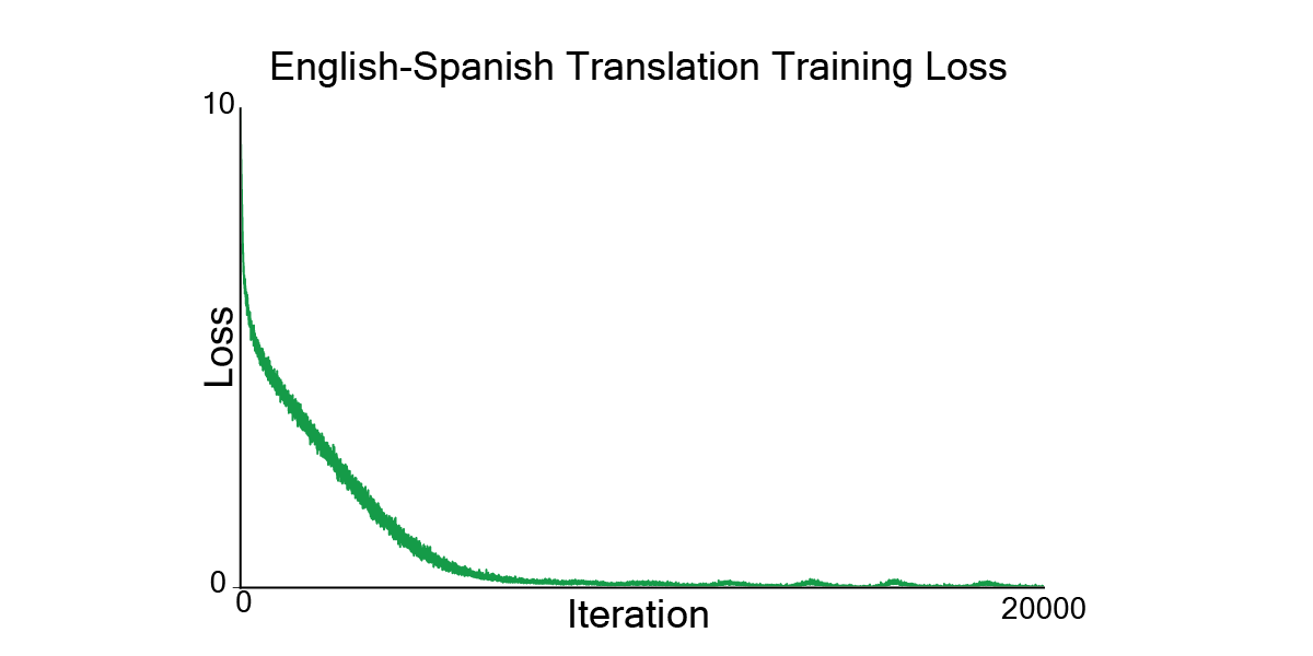
The code above is simple overview of the Vaswani et al., transformer architecture. I ran a much smaller model with parameters: $N = 3$, $h = 4$, $d_k = d_v = 32$, $d_{model} = h * d_v = 128$, $d_{ff} = 4 * d_{model} = 512$, $src_{vocab} = tgt_{vocab} = 10000$, $batch_{size} = 64$, $seq_{len} = 1000$, and trained for 20k iterations with a learning rate of $3e-4$. I used the hugging face opus books english-spanish translation dataset for training and testing. The code to to grab the translation data set can be found here: [TranslationData.ipynb]. The model I trained had 5,242,000 parameters, about 8% of the parameters of the original transformer base model (~64M Paramters). The code to run the model can be found here: [Transformer.ipynb] and the model is here : [Github - main.py]. I also included a helper function in main.py to test the model every 500 iterations.
    import torch
import torch.nn as nn
from torch.utils.data import DataLoader
from TranslationData import build_translation_datasets
from main import Transformer
import math

print('\n'*2)
train_dataset, test_dataset = build_translation_datasets(
    dataset_name="opus_books",
    lang_pair="en-es",
    src_lang="en",
    tgt_lang="es",
    max_len=32,
    max_vocab=10000,
    n_train=10000,
    n_test=1000
)
dataset = train_dataset
class Param:
    N: int = 3
    h: int = 4
    seq_len: int = dataset.seq_len
    d_k: int = 32
    d_v: int = d_k
    d_model: int = h * d_v
    d_ff: int = 4 * d_model
    init_scale: float = 0.02
    src_vocab_size: int = len(dataset.src_stoi)
    tgt_vocab_size: int = len(dataset.tgt_stoi)
    batch_size: int = 64
    iters = 20000
    lr: float = 3e-4
param = Param()
transformer = Transformer(param,dataset)

total_params = sum(p.numel() for p in transformer.parameters())
trainable_params = sum(p.numel() for p in transformer.parameters() if p.requires_grad)

print(f"Total params: {total_params:,}")
print(f"Trainable params: {trainable_params:,}")
Here are some examples across training. You can tell the early examples are fairly garbage, but get better as the loss decreases.
    Terminal Output:
--------------------------------------------------------------------------------
iteration 0, loss = 9.2182

SRC English:
the iron of lincoln island , as has been said , was of excellent quality , and consequently very fit for being drawn out .

TARGET Spanish:
el hierro de la isla lincoln , como es sabido , era de excelente calidad ; por tanto , muy fácil de <unk> .

PRED Spanish:
contrario <unk> recent recent recent recent recent recent recent recent recent recent recent recent recent recent recent puro francisco francisco francisco francisco recent recent puro recent puro recent recent recent recent


--------------------------------------------------------------------------------
iteration 1000, loss = 3.7032

SRC English:
the iron of lincoln island , as has been said , was of excellent quality , and consequently very fit for being drawn out .

TARGET Spanish:
el hierro de la isla lincoln , como es sabido , era de excelente calidad ; por tanto , muy fácil de <unk> .

PRED Spanish:
el <unk> , y , se <unk> , y , y , y , y , y , y , y <unk> a la <unk> .

--------------------------------------------------------------------------------
iteration 7000, loss = 0.1096

SRC English:
the iron of lincoln island , as has been said , was of excellent quality , and consequently very fit for being drawn out .

TARGET Spanish:
el hierro de la isla lincoln , como es sabido , era de excelente calidad ; por tanto , muy fácil de <unk> .

PRED Spanish:
el hierro de la isla lincoln , como es sabido , era de excelente calidad ; por tanto , muy fácil de <unk> .

--------------------------------------------------------------------------------
iteration 19000, loss = 0.0152

SRC English:
the iron of lincoln island , as has been said , was of excellent quality , and consequently very fit for being drawn out .

TARGET Spanish:
el hierro de la isla lincoln , como es sabido , era de excelente calidad ; por tanto , muy fácil de <unk> .

PRED Spanish:
el hierro de la isla lincoln , como es sabido , era de excelente calidad ; por tanto , muy fácil de <unk> .
Sources
- [1] Vaswani, A. et al. Attention Is All You Need. Preprint at https://doi.org/10.48550/ARXIV.1706.03762 (2017). [doi]
- [2] Hendrycks, D. & Gimpel, K. Gaussian Error Linear Units (GELUs). Preprint at https://doi.org/10.48550/ARXIV.1606.08415 (2016). [arxiv]
- [3] Elhage, et al., "A Mathematical Framework for Transformer Circuits", Transformer Circuits Thread, 2021. [Transformer Circuits]
- [4] Jimmy Lei Ba, Jamie Ryan Kiros, and Geoffrey E Hinton. Layer normalization. arXiv preprint arXiv:1607.06450, 2016. [arxiv]
← Back to Blog